Dissolution of a Single θ-Al2Cu Particle in FCC Matrix
Purpose: Learn to perform single-particle dissolution simulation.
Module: PanDiffusion
Thermodynamic and Mobility Database: AlCu_MB.tdb
Batch file: Example_#4.12.pbfx
Calculation Procedures:
-
Create a workspace and select the PanDiffusion module following Pandat User's Guide: Workspace;
-
Load AlCu_MB.tdb following the procedure in Pandat User's Guide: Load Database and select both two elements;
-
Click on the menu "PanDiffusion → Dissolution Simulation" or click the icon
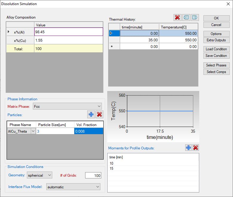
 and set up the calculation condition as shown in Figure 1;
 -
Click on “Select Phases” and make Fcc and AlCu_Theta the entered phases, while other phases are suspended;
-
In Alloy Composition set a composition of Al-1.55Cu (at%);
-
The total number of grids (# of Grids) is 100;
-
The Geometry of particles is set to “Spherical”;
-
In “Phase Information”, select Fcc as “Matrix Phase”.
-
To add a particle, click the blue “+” button in the "Particle" field, then select AlCu_Theta in “Phase Name”. “Particle Size” is set to 3.0 mm. “Vol. Fraction” is set to 0.008;
-
The “Thermal History” is a period of 35 minutes at 550°C;
-
Click OK to start calculation;
-
By default, dissolution simulation gives time-evolution of particle size as output. In order to display composition profile at desired moments, click the blue “+” button next to the “Moments for Profile Outputs” and input a time value. As shown in Figure 1, profiles at 10 minutes and 15 minutes will be outputted. Click OK to start calculation;
-
Details on these options can be found in Pandat User's Guide: Settings in Particle Dissolution Simulation.
Post Calculation Operation:
-
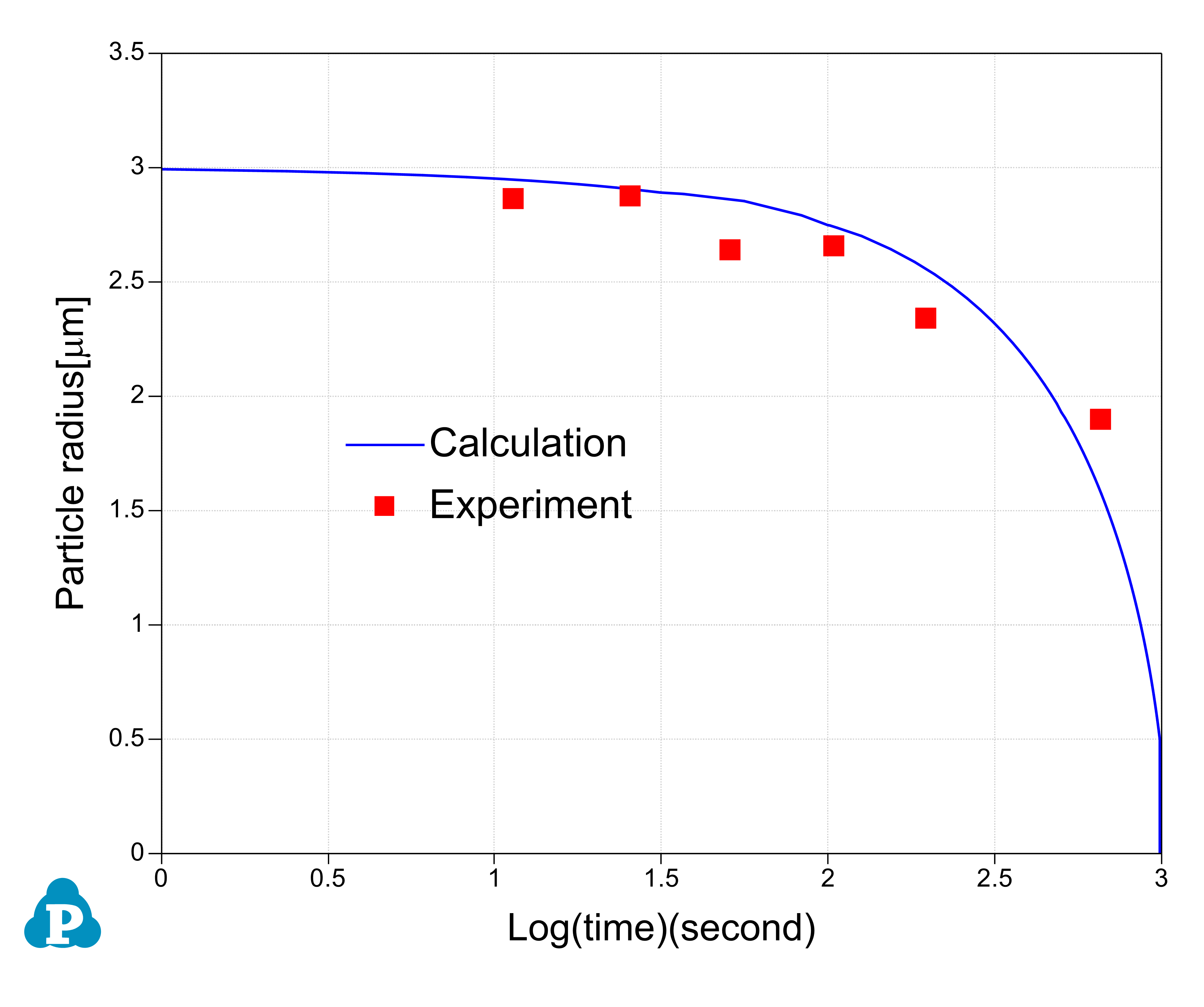
The calculated particle dissolution with time is shown in Figure 2 User can modify it by changing the title, the scale and so on from the Property Window. User can also add experimental data by clicking menu "Table → Import Table From Files", and select Example_#4.12.txt, and then follow Precipitation Simulation of Ni-14Al (at%) Alloy to add the experimental data on the plot. More information about change graph appearance can be found in Pandat User's Guide: Property.
-
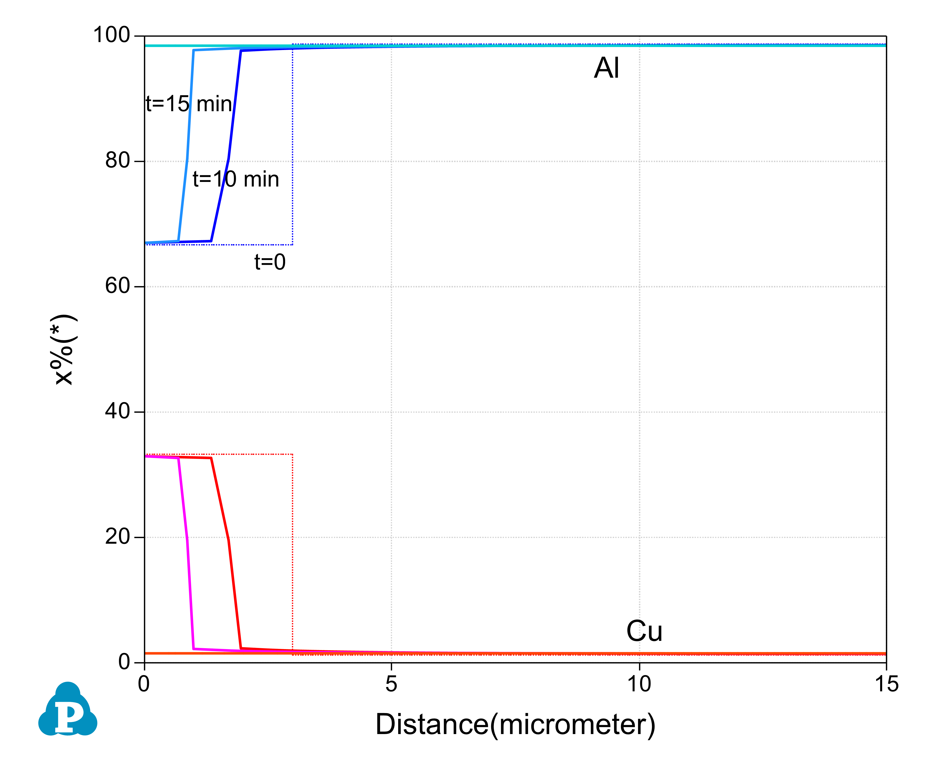
Click and open the Default table and select “distance”, “x%(Al)” and “x%(Cu)” to plot the composition profiles at starting, ending and the two selected intermediate times as shown in Figure 3.